The Build #001: Understanding the Data (CRISP-DM)
Your first hands-on session using a realistic IT dataset, designed to build practical AI intuition and set the foundation for future engineering exercises.

Welcome to the first edition of The Build, a weekly practical series created to help IT leaders and curious practitioners deepen their technical understanding of AI. In my recent skills gap article, I talked about why leaders benefit from getting closer to the mechanics of AI. When you understand what’s happening under the hood, your strategic thinking changes, your conversations improve, and you become far more credible when shaping AI direction inside the business.
This series exists to help you build that confidence one practical step at a time.
I’ve said many times that data is the starting point of AI. Universities treat it as foundational, most AI courses open with it, and nearly every real-world AI project begins with understanding the data before doing anything else. You’ll see why quickly. Without understanding your data, everything that follows becomes guesswork.
Over the coming weeks, we’ll work through practical exercises that mirror real AI engineering work: data exploration, feature creation, model behaviour, evaluation techniques, notebook workflows, and more. But before we ever talk about models, we have to start where every real AI project starts: with the data.
To do this properly, we’re going to anchor this edition in the CRISP-DM process, the same structured framework used by data scientists and AI teams across the industry.
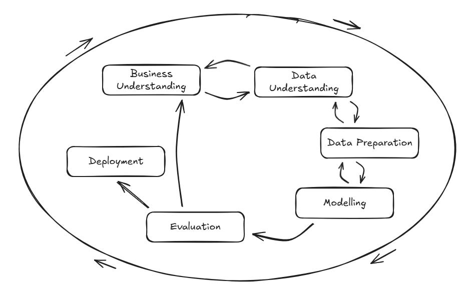
The Cross Industry Standard Process for Data Mining was developed by a consortium of companies involved in Data Mining (Chapman et al, https://www.scirp.org/reference/referencespapers?referenceid=1592779). Most people use some variation of this model, but it is foundational in that sense, and everyone agrees on the first three steps.
CRISP-DM lists the first three stages of any data or AI project as:
Business Understanding
Data Understanding
Data Preparation
Those first two steps occur before any technical work begins. We’ll cover business understanding, then move into more hands-on data understanding before moving into data preparation. Data preparation can be an exhaustive topic, so we’ll dig deeper into it as part of The Build series of articles.
To make this as realistic as possible, we’ll work with a synthetic yet life-like CSV dataset containing IT service desk records. This dataset is sufficiently large and diverse to support a range of practical applications. Over time, we’ll take this same dataset through the entire CRISP-DM lifecycle: exploration, preparation, modelling, evaluation, and deployment.
The data was generated with AI, so any similarity to real people, events, or that one time your service desk melted down on a Friday afternoon is purely coincidental.
For now, we’ll cover the importance of business understanding before taking the very first practical step: load the data, explore it, and understand what story it’s trying to tell.
Don’t worry if Jupyter, Python, or pandas are new to you. Everything will be explained clearly, and you’ll be able to follow along without any prior experience.
Business Understanding: CRISP-DM Step 1
Before touching a single line of code, we need to understand why we’re looking at this data and what problem we are trying to solve. CRISP DM starts with Business Understanding for a simple reason: without a clear purpose, even the most elegant analysis becomes meaningless.
We’re grounding this first Build in a familiar domain, the IT service desk. Because service desks are ubiquitous across most organisations, their data provides a realistic, relatable environment for learning core AI and data concepts.
This step focuses on connecting data to the real work of IT leadership. Service desk data reflects:
User friction and productivity loss
Operational bottlenecks
System reliability
Team workload and skills distribution
Service quality and customer experience
Potential risks brewing beneath the surface
In short, this dataset represents the day-to-day operational heartbeat of IT. And as an IT or AI tech leader, you likely already have a strong intuitive sense of this landscape. That’s useful, but it won’t always hold in other business domains. In finance, logistics, marketing, HR, procurement, or CX, you may not instinctively understand why specific data exists or what influences it.
That’s why Business Understanding matters. When you’re in an unfamiliar domain, your first step is always to speak with people who live that process daily. Their knowledge shapes the questions you ask and prevents you from misinterpreting the data.
For service desk data, typical leadership questions include:
Where are we seeing the most operational friction?
Which teams are under pressure and why?
Are we meeting service expectations?
What problems are emerging that we haven’t spotted yet?
Which areas or departments consistently generate the most demand?
These questions provide direction and help us stay anchored as we move deeper into the technical stages of CRISP-DM.
Data Understanding: CRISP-DM Step 2
With a clear purpose established, we move into Data Understanding, the stage where we begin exploring what the dataset contains. This isn’t about fixing anything yet. It’s about becoming familiar with the raw material.
Think of this as the reconnaissance phase. You’re not drawing conclusions; you’re building intuition.
At this stage, leaders and analysts should be asking themselves:
What kinds of data do we have? Dates, categories, text, numbers?
Is the dataset complete? Are there missing values or inconsistent fields?
How is the data distributed? Are some categories dominant? Are some rarely used?
What early patterns stand out? Do some departments log far more tickets? Are specific priorities overused?
Does anything look unusual or suspicious? Strange timestamps, oddly frequent categories, or priority patterns that don’t match real-world experience.
Data Understanding is about seeing the data as it really is, not how we expect or want it to be. This step helps you:
Spot problems early (inconsistencies, missing values, odd behaviour).
Identify which parts of the dataset will matter most later.
Develop a mental model of what the analysis or AI model may reveal.
Avoid costly mistakes in interpretation.
By clarifying the terrain, we set ourselves up for the next stage: Data Preparation, where we begin shaping and refining the dataset to make it meaningful, reliable, and ready for deeper exploration.
Now that we’ve grounded ourselves conceptually, we can move on to the practical exploration of the dataset.
Downloadable Resources
To follow along, you will need:
service_desk_dataset.csv, the full synthetic dataset
the_build_001.ipynb, notebook with exploration steps
Step 1. Introducing the Dataset
Here is the dataset we’ll use throughout The Build series. It contains thousands of synthetic service desk tickets designed to resemble real organisational data. This version has been deliberately created with richness, imperfections, and inconsistencies, because real-world data is rarely clean. These imperfections provide ample opportunities for data cleansing, transformation, simplification, and feature engineering.
Below is a summary of all dataset columns to help you quickly understand what each feature represents and how it will be used throughout this series.
Ticket Metadata
ticket_id
Unique identifier for each ticket.
opened_datetime
Timestamp when the ticket was created.
closed_datetime
Timestamp when the ticket was resolved (may be missing).
sla_target_hours
Allowed resolution time based on ticket priority.
reopened
Indicates whether the ticket was reopened after closure.
User and Department Information
user_department
Department of the user, including intentional spelling mistakes and variations.
user_role
User’s role or seniority (Employee, Manager, Director, Executive, Contractor).
customer_type
Whether the user is Internal or External.
location
Office or region. Includes duplicates such as Manchester and Manchester Office.
Ticket Classification
priority
Importance of the ticket (Low, Medium, High, Critical).
urgency_level
Secondary urgency measure (Low, Medium, High, Severe).
issue_severity
Severity rating (1 - Critical, 2 - High, etc.).
category
Issue type (Password reset, VPN problem, Application error, etc.).
system_affected
Business or technical system impacted (Email, CRM, HR System, etc.).
device_type
Device involved (Laptop, Desktop, Mobile, Tablet, Virtual Machine).
Operational Handling
assigned_team
Team responsible for handling the issue.
channel
Method used to raise the ticket (Email, Phone, Portal, Chat).
ticket_source
Additional source detail (Walk-in, Monitoring Alert, Self-Service).
follow_up_required
Indicates whether further action is needed after closure.
resolution_notes
Short summary of the resolution outcome.
Text Content
ticket_description
Free-text description of the issue. Useful for natural language processing.
Asset and System Metadata
asset_id
Identifier for the affected device or system component.
Step 2. Installing Jupyter
Before we jump into installation, it’s worth explaining what Jupyter is and why it’s widely used in both business and academic settings.
What is Jupyter?
Jupyter is an interactive environment that lets you write and run code in small, manageable blocks called cells. Each cell can contain Python code, text, visuals, tables, or charts. Instead of writing a complete program and running it all at once, Jupyter lets you iterate step by step, see results immediately, and experiment quickly.
Think of it as a digital lab notebook for data work.
Why is Jupyter so popular?
Jupyter has become the default tool for:
Data science: Analysts, engineers, and AI practitioners use it to explore data, test ideas, and build models.
Machine learning experimentation: Most model prototypes start life in a Jupyter notebook because it’s fast to iterate.
Business analytics: Dashboards, reports, and exploratory analysis often begin in Jupyter before being handed off to BI tools.
Academia and research: Universities use Jupyter to teach programming, statistics, AI, and scientific computing because it’s beginner-friendly and powerful.
Reproducibility and collaboration: A notebook shows not only the final output but also every step required to get there. This makes work easy to review, share, and explain.
Why are we using Jupyter in The Build?
Because it is:
Beginner-friendly – you can run one cell at a time.
Immediate – you see results instantly.
Flexible – perfect for combining explanations, code, and outputs.
Industry standard – if you learn Jupyter, you’re learning in the same environment as data scientists and AI engineers.
You don’t need prior experience. By the end of this series, you’ll be comfortable running Python, exploring data, and building your own workflows inside a notebook.
We can now discuss how to install it.
Installing Jupyter
Before we load any data, you’ll need a working Jupyter environment. The easiest and most common way to get Jupyter running on your machine is through Anaconda, which packages Python, Jupyter Notebook, and many useful scientific libraries into a single installer.
Rather than walk through the installation step by step for each operating system (Windows, macOS, and Linux), the most reliable approach is to follow Anaconda’s official guides. These guides are regularly updated and tailored to your specific OS.
You can find them here:
Official Anaconda Installation Guides
https://www.anaconda.com/download
Choose your operating system, follow the steps, and once installed, you’ll be able to launch Jupyter Notebook directly from the Anaconda Navigator.
Once Jupyter is installed and running, we can begin working with the dataset.
Step 3. Load the Data in Jupyter
Let’s start to get our hands dirty. The key here is not to panic if Jupyter is new to you. It is simple to learn, and we will keep this first session deliberately light. You are encouraged to experiment, break things, and re-run cells. That is often the best way to learn.
Open a Jupyter Notebook and run the following by clicking inside the cell and pressing Ctrl+Enter if you’re using Windows (or the equivalent key combination for your operating system):
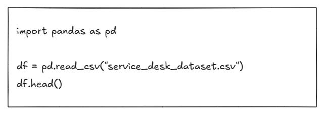
What this does
import pandas as pd- loads the pandas library, which gives us powerful tools for working with tabular data.df = pd.read_csv(”service_desk_dataset.csv”)- reads the CSV file into a DataFrame calleddf.df.head()- displays the first five rows, allowing you to visually confirm that the data has loaded correctly.
How to interpret the output
You should see a small preview of your dataset, with column names across the top and a few rows below. This is your first chance to spot:
Obvious errors
Strange or unexpected values
Missing timestamps
Odd-looking departments, locations, or categories
Please don’t worry about fixing anything yet. At this stage, we are simply getting familiar with the shape and feel of the data.
Step 4. Explore the Data
Understanding your dataset means asking the simplest possible questions first. In this step, we are not trying to build models or produce polished reports. We are just trying to understand what we are dealing with.
How big is it?

What this does
Returns a tuple in the form (rows, columns).
How to interpret it
If you see (1500, 25), it means 1,500 records and 25 features. This tells you:
There is enough data to see patterns.
There are plenty of features to work with.
Cleansing and preparation will matter.
What types of data does it contain?

What this does
Shows each column, its data type, and how many non-null values it contains.
How to interpret it
This is one of the most critical early commands. You can quickly see:
Which columns have missing values
Which columns are stored as text when they might represent dates or numbers
Whether any fields look suspicious (for example, a column that is almost entirely empty)
This is often where data quality issues first reveal themselves.
What do the numbers look like?

What this does
Produces summary statistics for numeric columns: count, mean, standard deviation, minimum, maximum, and common percentiles.
How to interpret it
Look for:
Very large spreads between minimum and maximum values
Unusual averages
SLA targets or numeric fields that do not look realistic
This gives you a sense of whether the numbers in your dataset behave as you would expect.
What are the most common categories?

What this does
Shows the most common values in the category column.
How to interpret it
This helps you understand:
The types of issues users most frequently report
Where operational pressure may be highest
Which categories might be worth simplifying or grouping later
This kind of simple frequency analysis is often enough to start useful leadership conversations.
This is the heart of the Data Understanding stage in CRISP-DM: examining the data as it is, not as you assume it should be. No cleaning yet. No assumptions. No transformations. You are simply learning what you have.
Step 5. Early Observations
When you explore a new dataset, you should start forming observations such as:
Are specific departments logging far more tickets?
Are priorities evenly distributed or skewed?
Are some categories extremely rare or extremely common?
Are there fields that look incomplete or inconsistent?
Do timestamps look valid and complete?
These aren’t conclusions, only early impressions. But they matter because they guide the next CRISP DM stage: data preparation.
Next week’s Build will take this dataset further by preparing and simplifying the features so we can begin extracting insights.
Downloadable Resources
To follow along, you will need:
service_desk_dataset.csv, the full synthetic dataset
the_build_001.ipynb, notebook with exploration steps
Many AI projects fail not because the model is poor, but because the data was never appropriately understood in the first place. CRISP-DM prioritises data understanding over preparation, modelling, or experimentation. Everything that happens later, the insights, the predictions, the automation, even the storytelling, depends on the quality of thinking you apply here.
If you can understand the data, you can understand the problem. Once you understand the problem, every decision downstream becomes clearer. You know what to clean. You know what to transform. You know which features matter. You know which questions are worth answering. Without that foundation, even the best tools and algorithms will struggle to deliver value.
This first edition of The Build may feel gentle, but it sets the tone for everything that follows. You’ve taken the same first steps as data scientists, analysts, and AI engineers on real projects: grounding the work in a business context, exploring raw data, and forming early intuition about what’s happening beneath the surface.
That intuition doesn’t just make you better at working with AI; it makes you better at leading the people who work with AI.
Strong leadership in AI isn’t about out-coding your data scientists or being the technical expert in every conversation. It’s about understanding enough of the process to:
Ask sharper, more relevant questions.
Challenge assumptions with confidence.
Spot risks earlier.
Understand what “good” looks like in analysis and modelling.
Provide clearer direction to business analysts and data scientists.
Build trust by speaking their language without overwhelming them with detail.
When you understand the early stages of CRISP DM, especially Business Understanding and Data Understanding, you see the world through the same lens your analysts and data scientists do. You appreciate the complexity they manage, the constraints they navigate, and the thinking behind their recommendations. This builds stronger collaboration, sharper decision-making, and far more effective leadership.
Next week, we move into Data Preparation, the stage where the dataset stops being something you look at and becomes something you shape. We’ll clean the data, engineer useful features, simplify complexity, and prepare the foundation for more advanced techniques in future Builds.
This is where the raw material starts turning into something powerful.